数学代写| R语言考试代写

Tidy Data, Plotting, Stats, Linear Regression, Logistic regression

R语言考试代写

1. - 考题 Sample(只有几题有解答)

$\# 1$

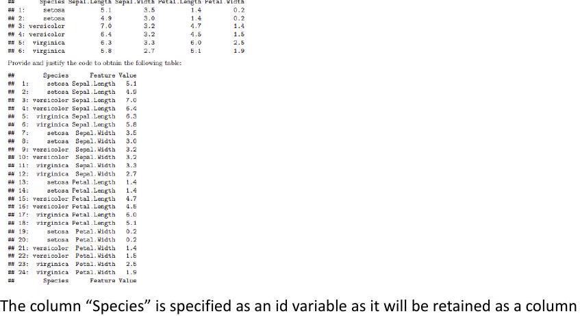
Given a suluct of the iris dataect consisting of two observations of teach species:

Iris_dt $<-$ as, data,table(iris)

Iris_dt <- as, data,table(iris)
iris_sub <- iris_dt [, .SD[1:21, by = Species]
iris_sub

iris_sub

Spacic
setos
setosa
$\mathrm{~ s e t e r}$


H. 2: Setosa
#7. 3: vereicolor
$\mathrm{~ a t ~ 4 a ~ v e}$

an b: virginic

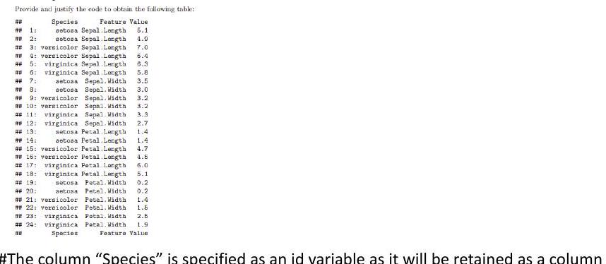
in the melted table. The previous column names are flattened into a new column “Feature” and the previous values are stored in a new single column “Value”.

melt(iris sub, id.vars = ‘Species’, variable.name = ‘Feature’, value.name = ‘Value’)

2. #2

The greenhouse gases dataset from the dslabs package contains the concentration of the 3 gases $\mathrm{CH} 4, \mathrm{CO} 2$ aud $\mathrm{N} 20$, measured crery 20 ycars since the year $0 .$ Read it using: gg_dt <- as. data. table (dslabs: igreenhouse_gases). Write the R code which produces the following plot using the library grplot2. Matching the exact rendering style (font, font size, choice of color) is not required.


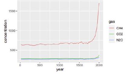
$\operatorname{ggplot}\left(g g_{-} \mathrm{dt}\right.$, aes(year, concentration, color=gas)) $+$ geom_line () $\# 3$

We consider a linear regression model parameterized as
$$y_{i}=\alpha+\beta \cdot x_{i}+\epsilon_{i}$$

the response variable, $\alpha$ and $\beta$ the coefficients, $x_{i}$ the explanatory variable

where $i=1 \ldots N$ denotes the data point indices, $y_{i}$ is the response variable, $\alpha$ and
and $\epsilon_{i}$ the error term. Let $\hat{y}_{i}$ be the i-th fitted value and $\epsilon_{i}$ be the i-th residual.

and $\epsilon_{i}$ the error term. Let $\hat{y}_{i}$ be the i-th fitted value and $\epsilon_{i}$ be the i-th residual.
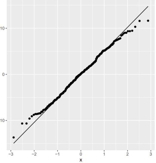
Does the following plot provide evidence against the assumptions of the linear regression? Instify. (1 point for the correct.

Does the following plot provide evid
answer and the correct justification.)


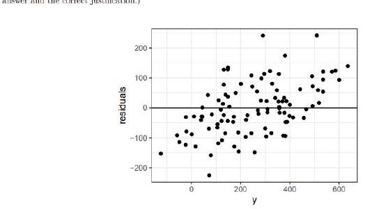
Linear regression assumes independence between error and predicted value, y_hat, but not between the error and the response, $y$. This plot does not show evidence against the assumptions of linear regression.

$\# 4$


#5

The adrissions dataset from the dislabs package contains admissions data for six mejors split by geader.

data(admissions)

head (admissions)

#H najor gender admitted applicants



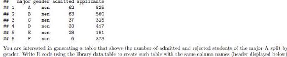
## gender major admitted status cases

#H 1: mon $\quad$ mender major admitted_status cases

$\begin{array}{lllr}\text { ## 2: women } & \text { A } & \text { admitted } & \text { B2 } \\ \text { ## 3: men A } & \text { rejected } & 763\end{array}$

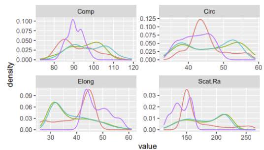
$\begin{array}{lllll}\# \text { # 3: } & \text { men } & \text { A } & \text { rejected } & 763 \\ \text { #H 4: women } & \text { A } & \text { rejected } & 26\end{array}$ The Vehicle dataset from the mlbench package contains different car silhouette features of 4 different types of cars.


Vehicle <- as, data, table (Vehicle)

head (Vehicle)

## Comp Circ D. Circ Rad. Ra Pr.Axis. Ra Max. L. Ra Scat. Ra Elong Pr. Axis.Rect

## 1: $\quad 95 \quad 48 \quad 83 \quad 178 \quad 72 \quad 10 \quad 162 \quad 42 \quad$ Max.L.Ha Scat.Ra Elong Pr.Axis.Rect

$\begin{array}{llllll}\text { ## } & 2: & 91 & 41 & 84 & 141\end{array}$

$\begin{array}{rrrrrrrrrrrr}\text { ## } & 3: & 104 & 50 & 106 & 209 & 66 & 10 & 207 & 32 & 23 & 149 \\ \text { ## } & 4: & 93 & 41 & 82 & 159 & 63 & 9 & 144 & 46 & 19 \\ \text { ### } & 5: & 85 & 44 & 70 & 205 & 103 & 52 & 149 & 45 & & 19\end{array}$

$\begin{array}{llccccccc}\text { ## } 6: & 107 & 57 & 106 & 172 & 50 & 6 & 255 & 26 \\ \text { ## } & \text { Max. L. Rect } & \text { Sc. Var Maxis Sc.Var.maxis Ra Gyr } & \text { Skew.Maxis Skenmaxis Kurt.maxis }\end{array}$

## Max.L. Rect Sc. Var.Maxis Sc.Var.maxis Ra. Gyr Skew. Maxis Skew.maxis Kurt.maxis

$\begin{array}{lllllllll}\text { ### } & 1: & 159 & 176 & 379 & 184 & 70 & 6 & 16 \\ \text { ## } & 143 & 170 & 330 & 158 & 72 & 9 & 14\end{array}$

$\begin{array}{llllllrrrr}\text { ## } & 2: & 143 & 170 & 330 & 158 & 72 & 9 & 14 \\ \text { ## } & 3: & 158 & 223 & 635 & 220 & 73 & 14 & 9 \\ \text { ## } & 4: & 143 & 160 & 309 & 127 & 63 & & 6 & 10 \\ \text { # } & 5: & 144 & 241 & 325 & 188 & & 127 & & 9 & \end{array}$

$\begin{array}{rrrrrrrrrrr}\# \# 5: & 144 & 241 & 325 & 188 & 127 & 9 & 11 \\ \# 6: & 169 & 280 & 957 & 264 & 85 & 5 & 9\end{array}$

$\begin{array}{cc}169 & 280 \\ \text { Kurt Maxis Holl. Ra Class }\end{array}$

Kurt.Maxis Holl. Ra Class

$\begin{array}{llll}\text { ## } 1: & 187 & 197 & \text { van } \\ \text { ## } 2: & 189 & 199 & \text { van }\end{array}$

$\begin{array}{lllr}\text { ## 2: } & 189 & 199 & \text { van } \\ \text { ## 3: } & 188 & 196 & \text { saab }\end{array}$

$\begin{array}{lllr}\text { ## } 3: & 188 & 196 & \text { saab } \\ \text { ## } 4: & 199 & 207 & \text { van }\end{array}$

$\begin{array}{llll}\text { ### } & 4: & 199 & 207 & \text { van } \\ \text { # } & 180 & 183 & \text { bus }\end{array}$

## 6: $\quad 181 \quad 183$ bus

Write R using the library ggplot2 code that produces the following plot.

Class

opel

yan
value
You are interested in testing whether 2 friends have independent tastes for movies. You ask each of them their opinion about
100 movies and obtained the following observations (just the header shown):
You are interested in testing whether 2 friends have independent tastes for movies. You ask each of them
100 movies and obtained the following observations (just the header shown):

$\# 7$

## movie friend1 friend2

1 Like Dislike

2 Dislike Dislike

3 Dislike Dislike

5 Dislike Dislike
6 Dislike Like

6: 6 a permutation approach to test it. We consider as alternative hypothesis that the two friends have similar movie tastes.

Fill in the code and explain what each of the two code chunks does.

t_obs <- dt[friend1 = friend2, .N] # value of the statistic in observed dataset $N_{-}$permu <- 999

# number of permutated datasets

$t_{\text {star }}<$ – numeric $\left(N_{\text {permu) }}\right.$ # value of the statistic in pernuted datasets

for (i in 1:N permu)f

for 1 in
#HCode $A:$

# $t_{-} 3 \operatorname{tar}[t]<-$

#H Code B: Compute two-sided P-value. Stare it in variable pval:

3. - 平时练习题 example

$\# 1$

1. Reproduce the following visualization of the association between the variables cty and hwy for the years 1999 and 2008 from the dataset mpg using the library ggplot2:

data $(\operatorname{mpg})$

$m p g<-a s \cdot$ data.table $(m p g)$

ggplot (mpg, aes (cty, hwy, color=factor (year))) + geom_point() + geom_smooth(method= $\left.^{4} 1 \mathrm{~m}^{2}\right)$


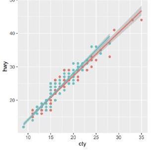
factor(year)

1999
2008

2008

2. #2

To start, read the provided heights dataset using the following line of code (it’s your own heights data):

heights <- fread(“extdata/height. $\left.\operatorname{csv}^{\prime \prime}\right) \%>\%$ na. omit() $\%>$

– [, sex:=as.factor(toupper $($ sex $))]$

heights

1. Predict each student’s height, given their sex and their parents heights.

$m<-$ heights $[$, Im(height sex + mother + father) ]

summary (m)

## Call:

## $\operatorname{lm}$ (formula $=$ height $-$ sex $+$ mother $+$ father)

##

## Residuals:

## Min 1Q Median $3 Q$ Max

$\begin{array}{lllllll}\# \# & -13.6777 & -3.5802 & 0.1564 & 3.3738 & 11.6338\end{array}$

\# Coefficients:

Estimate Std. Error t value Pr $(>|t|)$

$\# \#$ (Intercept) $42.07027 \quad 8.77308 \quad 4.7952 .80 e-06 * * *$

## sexM

$14.00534$

$0.60830$


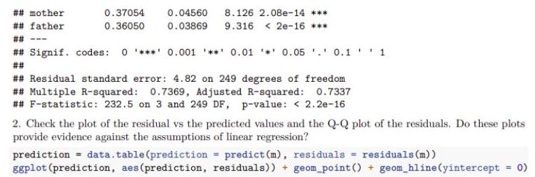
## mother $0.370540 .04560 \quad 8.1262 .08 e-14 * * *$

## father $\quad 0.36050 \quad 0.03869 \quad 9.316<2 e-16 * * *$


## Signif. codes: 0 ‘***’ $0.001^{\prime} * *^{\prime} 0.01^{\prime} *^{\prime} 0.05,^{\prime} 0.1,1$

##葉

## Residual standard error: $4.82$ on 249 degrees of freedom

## Multiple R-squared: $0.7369$, Adjusted R-squared: $0.7337$

## F-statistic: $232.5$ on 3 and 249 DF, p-value: $<2.2 \mathrm{e}-16$

2. Check the plot of the residual vs the predicted values and the Q-Q plot of the residuals. Do these plots provide evidence against the assumptions of linear regression?

prediction $=$ data.table(prediction $=$ predict $(\mathrm{m})$, residuals $=$ residuals $(\mathrm{m}))$

ggplot (prediction, aes(prediction, residuals)) + geom_point() + geom_hline(yintercept =

$-10$

$10-$

0

ggplot (prediction, aes (sample = residuals)) + geom_qq() + geom_qq_line

ggplot (prediction, aes (sample = residuals)) + geom_qq () + geom_qq_line()


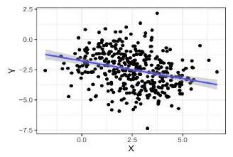
When visualizing the relationship between the variables $X$ and $Y$, we can observe a negative correlation between $\mathrm{X}$ and $\mathrm{Y}$ :

ggplot(data, aes $(\mathrm{X}, \mathrm{Y}))+$ geom_point ()$+$ geom_smooth $\left(\mathrm{method}=1 \mathrm{~lm}^{\prime}\right)+\mathrm{mytheme}$


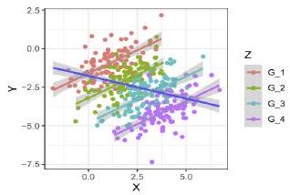
However, when grouping by the variable Z we observe a positive correlation which is the opposite direction as before:

ggplot(data, $\operatorname{aes}(\mathrm{x}=\mathrm{X}, \mathrm{y}=\mathrm{Y}))+$

geom_point (aes (color $=$ Z) ) +

geom_smooth $(\mathrm{aes}(\mathrm{color}=Z)$, method $=” 1 \mathrm{~m} “)+$

geom_smooth(method $\left.=11 \mathrm{~lm}^{\prime \prime}\right)+$ mytheme


$\# 4$

The growth table contains the growth rates expressed in generations per day for each strain in five different growth media. These growth media are YPD (glucose), YPD_BPS (low iron), YPD_Rapa (Rapamycin), YPE (Ethanol), YPMalt (Maltose).


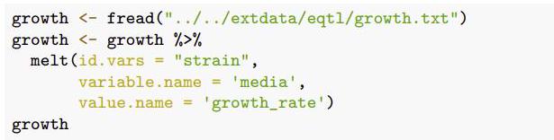
growth <- fread(“../../extdata/eqtl/growth.txt”)

growth <- growth \% \%

melt(id. vars = “strain”,

variable.name = ‘media’,

value. name $=$ ‘growth_rate’ )

growth

## strain media growth_rate

## 1: seg_01B YPD 12.603986

$\begin{array}{lllll}\# \# & 1: & \text { seg_01B } & \text { YPD } & 12.603986 \\ \# \# & 2: & \text { seg_01C } & \text { YPD } & 10.791144\end{array}$

## $\quad$ 3: seg_01D $\quad$ YPD $\quad 12.817268$

$\begin{array}{llll}\# \# & \text { 3: seg_O1D } & \text { YPD } & 12.817268 \\ \text { ## } & \text { 4: seg_02B } & \text { YPD } & 10.299210\end{array}$

$\begin{array}{lllll}\text { ## } & 4: & \text { seg_02B } & \text { YPD } & 10.299210 \\ \text { ## } & 5: \text { seg_02C } & \text { YPD } & 11.132778\end{array}$

## $\quad 5:$ seg_02C $\quad$ YPD $\quad 11.132778$

## 786: seg_49A YPMalt $\quad 4.592395$

## 787: seg_49B YPMalt

## 788: seg_50A YPMalt $\quad 4.303382$

## 789: seg_50B YPMalt $\quad 6.583852$

## 790: seg_50D YPMalt $\quad 7.421968$ To assess this hypothesis, we first create a data table called dt that contains the relevant data.


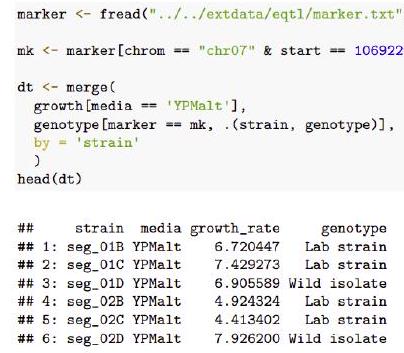
marker <- fread(“../../extdata/eqtl/marker.txt”)

mk <- marker[chrom $==”$ chr07″ \& start $==1069229$, id]

dt $<-\operatorname{merge}($

growth [media == ‘YPMalt’],

genotype [marker == mk, (strain, genotype)],

head (dt)

## strain media growth_rate genotype

## $1:$ seg_01B YPMalt $6.720447$ Lab strain

## 2: seg_01C YPMalt $7.429273$ Lab strain

## 3: seg_01D YPMalt $6.905589$ Wild isolate

## 4: seg_o2B YPMalt $\quad 4.924324 \quad$ Lab strain

## 5: seg_02C YPMalt $\quad 4.413402 \quad$ Lab strain

## 6: seg_02D YPMalt $\quad 7.926200$ Wild isolate

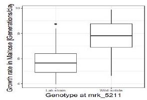
Genotype at that marker indeed associates with a strong difference in growth rates in the Maltose media, with a difference between the medians of $2.17$ generations per day.


$\mathrm{~ T r o b s ~ s t a d t ~ [ g e n o t y p e ~ a ~}$

T_obs <- dt [genotype == Wild isolate’, median(growth_rate, na
dt [genotype == ‘Lab strain’, median(growth_rate, na. rm=T)]


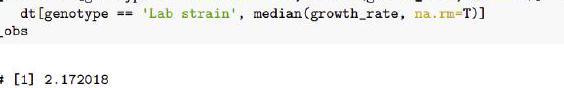
T_obs

[1] $2.172018$

R语言考试代写请认准UpriviateTA. UpriviateTA为您的留学生涯保驾护航。