PSTAT 120C: Data analytic report 1
Due: Nov 2, 2021 before class
Please submit your report as a pdf, word or image file. Please submit your $\mathrm{R}$ code in separate file(s). Please attach figures from R to illustrate your answers.

2. Suppose I want to estimate $E[Y \mid X]$ (the regression function). Is it possible to make the prediction risk (expected squared error) arbitrarily small by allowing our estimate $\hat{f}(X)$ to be more complex? While we can make training error arbitrarily small, making $f$ more complex may reduce bias at the expense of variance, and it does not effect the intrinsic error.
3. State two advantages of using leave one out cross validation (LOOCV) rather than K-fold CV.
1. LOOCV has lower bias as an estimate of prediction risk.
2. LOOCV may be easier to compute (closed-form if a linear smoother).
3. If there are categorical predictors, K-fold may “drop levels”. This is super weird/annoying. LOOCV is less likely to do this.
4. In cases where the interest is in using a linear model to predict future observations of the response variable, better results are obtained when the model includes all available explanatory variables. This last sentence is:
a. Always false
b. True only for continuous explanatory variables
c. True only for Gaussian noise
d. Always true
e. None of the above
None of the above. Results may be better or worse depending on the balance between bias and variance.
5. Using the trade off between variance and bias, explain why a more flexible linear regression model relative to least squares will give improved prediction accuracy.
“more flexible” means lower bias. The hope is that the decrease in bias will swamp any increase in variance and lead to lower expected MSE.
6. A former student says that we should always run LOOCV more than once and average the results. Why is this a bad idea?
LOOCV is not random, because every data point is always left out exactly once. So rerunning will give the same result (in contrast with K-fold).
7. Given a data set $y_{1}, \ldots, y_{n}$ the function $f: R \rightarrow R$ given by $f(a)=\frac{1}{n} \sum_{i=1}^{n}\left(y_{i}-a\right)^{2}$ is minimized at $a_{0}=\overline{y_{n}}$. The last sentence is:
a. always true
b. true only if $\overline{y_{n}} \geq 0$
c. true only if $\overline{y_{n}} \leq 0$
d. true only if $\sum_{i=1}^{n} y_{i}^{2} \leq \sum_{i=1}^{n}\left(y_{i}-\overline{y_{n}}\right)^{2}$
This is always true. $f$ is convex, taking the derivative, setting to 0 , and solving gives the solution.
8. In class we discussed leave one out cross validation (LOOCV) and its use as an estimator for the expected test error of a predictor $\widehat{f}$. Its formula is
$$
\mathrm{LOOCV}=\frac{1}{n} \sum_{i=1}^{n}\left(y_{i}-\widehat{f}^{(i)}\left(x_{i}\right)\right)^{2}
$$
Consider the following alternative estimator. Let’s call it lazy leave one out cross validation (LLOOCV):
$$
\mathrm{LLOOCV}=\frac{1}{n / 2} \sum_{i}^{n}\left(y_{i}-\widehat{f}^{(i)}\left(x_{i}\right)\right)^{2}
$$
For simplicity, we’ll assume that $n$ is even. These two estimators are the same except for the number of terms in the sum. How do the bias and variance of these two estimators compare to each other?
The bias is the same because the expected values are the same: $E\left[y_{1}-\widehat{f}\left(x_{1}\right)\right]$. The variance of LLOOCV is larger because there are half as many terms in the sum.
9. (Challenging) Suppose $Y_{1}, \ldots, Y_{n}$ are normally distributed with mean $\mu$ and variance $2 .$ I decide to estimate $\mu$ with the median of $Y_{1}, \ldots, Y_{n}$. Let’s call the median $M_{n}$. It turns out that the mean squared error of estimating $\mu$ with $M$ is
$$
E\left[\left(M_{n}-\mu\right)^{2}\right]=\frac{\pi}{n}
$$
What is the expected squared prediction error for $Y_{n+1}$
$$
E\left[\left(M_{n}-Y_{n+1}\right)^{2}\right]=? ? ?
$$
Prediction Error $=$ Estimation Error $+$ Irreducible Error (see Slide 03). So the answer is $\pi / n+2($ the variance of the irreducible error is 2).
10. (Challenging) Suppose I have 100 observations from the linear model
$$
Y_{i}=\beta_{0}+\sum_{j=1}^{p} x_{i j} \beta_{j}+\epsilon_{i}
$$
where $\epsilon_{i}$ is independent and identically distributed Gaussian with mean 0 and variance $\sigma^{2}$. I want to predict new observation $Y_{101} .$ I predict with $\widehat{Y}_{101}=0 .$ What is my expected test MSE?
$$
\operatorname{MSE}(0)=E\left[\left(Y_{101}-0\right)^{2}\right]=\operatorname{bias}^{2}(0)+\operatorname{Var}(0)+\operatorname{irreducible} \text { error }=\left(-\beta_{0}-\sum_{j=1}^{p} x_{101, j} \beta_{j}\right)^{2}+0+\sigma^{2}
$$
Alternatively, one could use:
$$
E\left[\left(Y_{101}-0\right)^{2}\right]=E\left[Y_{101}^{2}\right]=E\left[Y_{101}\right]^{2}+\operatorname{Var}\left(Y_{101}\right)=\left(\beta_{0}+\sum_{j=1}^{p} x_{101, j} \beta_{j}\right)^{2}+\sigma^{2}
$$
to get the same answer.
This question combined two concepts: the bias/variance/irreducible error decomposition with the definitions of bias and variance. Students last year found it very challenging.
1. Suppose $p=5$ and $n=100$. Give one reason to use ridge regression (with appropriately chosen $\lambda$ ) instead of OLS.
Two possible reasons are $(1)$ to avoid multicollinearity or (2) to decrease variance in the hope of improving prediction risk. Because you chose $\lambda$ appropriately, the ridge estimator has a lower estimate of expected test error.
2. Suppose $p=5$ and $n=100$. Give one reason to use OLS instead of ridge regression (with appropriately $\operatorname{chosen} \lambda)$. The best answer is “we want an unbiased estimator”. Related (and equally good) is “we want confidence intervals, p-values, etc.” In other words, all the things you learned about in Stat306 or CPSC 340 . You could try to argue that “we want lower bias in the hopes of improving prediction risk”. However, ridge regression with “appropriately chosen $\lambda “$ already accounts for this case. If OLS has a better risk estimate, then we will “appropriately” choose $\lambda=0$.
3. A disadvantage of “full trees” is that they “badly overfit”. Define “badly overfit”.
“Overfitting” means using an overly complicated model which has too much variance and not enough bias. That is the correct answer. You need not explain why trees do this, only define “overfitting”.
4. Suppose $y_{i}=f\left(x_{i, 1}, x_{i, 2}\right)+\epsilon_{i}$ for $i=1, \ldots, 100 .$ I try two methods to estimate $f$ :
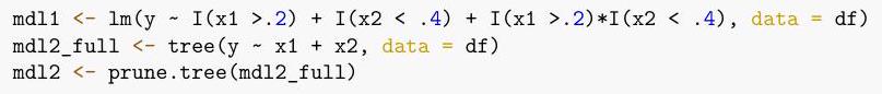
mdl1 $<-\operatorname{lm}(\mathrm{y} \sim \mathrm{I}(\mathrm{x} 1>.2)+\mathrm{I}(\mathrm{x} 2<.4)+\mathrm{I}(\mathrm{x} 1>.2) * \mathrm{I}(\mathrm{x} 2<.4)$, data $=\mathrm{df})$
mdl2_full <- tree (y x1 + x2, data = df)
mdl2 $<-$ prune.tree (mdl2_full)
It turns out that mdl2_full has 11 terminal nodes, while my pruned tree, mdl2, has four terminal nodes.
a. Based on the above information, how many parameters does mdl1 have?
b. Based on the above information, how many parameters does mdle have?
c. Based on the above information, which of mdl2_full or mdle has higher bias or can you not determine?
d. Based on the above information, which of mdl2_full or mdle has higher variance or can you not determine?
e. Based on the above information, which of mdl1 or mdle has higher bias or can you not determine?
f. Based on the above information, which of mdl1 or mdle has higher variance or can you not determine?
a. mdl1 has 4 parameters: intercept plus 3 slope coefficients.
b. mdl2 has 8 parameters: 4 splits (defining the 4 nodes) $+4$ averages within the nodes.
c. mdle has higher bias.
d. mdl2_full has higher variance.
e. mdl1 has higher bias
f. mdle has higher variance.
5. Define what it means for a regression method to be a “linear smoother”.
“linear smoother” means that there exists some matrix $\mathbf{S}$ such that the fitted values (in-sample predictions) $\widehat{\mathbf{y}}$ can be produced by the formula $\widehat{\mathbf{y}}=\mathbf{S y}$.
6. Suppose I estimate both ridge regression and lasso regression on some data with $\mathrm{n}=100$ and $\mathrm{p}=1257$. For lasso, the CV error at lambda.min=0.013 is 10.3. For ridge, the CV error at lambda.min $=0.02$ is 8.7. The lasso fit has 15 nonzero values of $\hat{\beta}$.
a. How many nonzero values of $\hat{\beta}$ does ridge regression have?
b. Which model has lower bias or can you not determine?
c. Which model should you use to predict future data or can you not determine?
d. Based only on the above information, would you say that it is more likely than not that the best linear model (without making any transformations) has a small number of true features or a large number of true features? Justify your answer. a. Almost certainly $1257 .$ (While possible to have a handful of zeros, it is highly unlikely for $\lambda<\infty$.
b. Cannot determine.
c. Ridge regression. It has the lower estimate of expected test error.
d. More likely that it has a large number. Ridge regression has the lower estimate of expected test error, and it uses all the features.
1. Suppose $y \in\{0,1\}$, and $x \in \mathbb{R}^{p}$ but instead of estimating logistic regression, I just estimate ordinary least squares using my data. Which of the following statements are true?
a. $\hat{\beta}$ is unbiased.
b. the confidence intervals produced have the correct coverage
c. $\hat{y}$ may take values outside of $[0,1]$
d. the residual sum of squares is the smallest relative to all other linear models (by “all other” I mean “linear models in these p covariates” no basis expansions, no additional covariates)
e. (somewhat challenging) the residual sum of squares is smaller than if I had used logistic regression
a. FALSE.
b. FALSE.
c. TRUE.
d. TRUE.
e. FALSE. (at least “not definitely true”) This one took some thinking on my part. But imagine $p=1$, and think about (c). OLS will make huge errors at very large and very small values of $x$, while the predictions from logistic regression are forced to be between 0 and $1 .$
2. Consider a classification problem with 2 classes and a 2-dimensional vector of predictor variables. Assume that the class conditional densities are Gaussian with mean vectors $\mu_{1}=(1,1)^{\top}$ and $\mu_{0}=(-0.5,-0.5)^{\top}$ and common covariance matrix $\Sigma=\left[\begin{array}{cc}1 / 2 & 0 \\ 0 & 1 / 4\end{array}\right]$. Recall that the density of a multivariate Gaussian random variable $W$ in $p$ dimensions with mean $\mu$ and covariance $A$ is given by
$$
f(w)=\frac{1}{(2 \pi)^{p / 2}|A|^{1 / 2}} \exp \left(-\frac{1}{2}(w-\mu)^{\top} A^{-1}(w-\mu)\right) .
$$
Suppose $\operatorname{Pr}(y=1)=0.75 .$ To which class would the Bayes Classifier assign the point $x=(.5, .5)^{\top} ?$
a. Class 1
b. Class 0
c. We do not have enough information to answer.
d. $\operatorname{Pr}(Y=1 \mid X=x)=\operatorname{Pr}(Y=0 \mid X=x)=1 / 2$ (we’re indifferent, so flip a coin)
Class 1 (a) is correct. We have $f_{1}(x)>f_{0}(x)$ so this would be true even if $\operatorname{Pr}(Y=1)$ were smaller than .5 (you’d have to calculate the values to see this)
3. Consider a classification problem with 2 classes and a $p$-dimensional vector of predictor variables. Assume that the class conditional densities are Uniform over the set $[0,2]^{p}$ (for class 1 ) and $[1,3]^{p}$ (for class 0 ). Suppose $\operatorname{Pr}(y=1)=0.75$. To which class would the Bayes Classifier assign the point $x=(1.5, \ldots, 1.5)^{\top} ?$
a. Class 1
b. Class 0
c. We do not have enough information to answer.
d. $\operatorname{Pr}(Y=1 \mid X=x)=\operatorname{Pr}(Y=0 \mid X=x)=1 / 2$ (we’re indifferent, so flip a coin) Still Class 1 (a). Now $f_{1}(x)=f_{0}(x)$, but the prior on Class 1 is higher. (See here for the specific formula for this and the previous question.)
4. TRUE/FALSE. Logistic regression makes fewer assumptions about the joint distribution of $(Y, X)$ than LDA does.
TRUE. See here. Logistic regression assumes a form for $P(Y=1 \mid X=x)$ but leaves the remainder unmodelled.
5. TRUE/FALSE. It is not possible to have a non-linear decision boundary with logistic regression.
FALSE. Can just use basis expansion, see here
6. TRUE/FALSE. Logistic regression does not perform variable selection.
True (could use lasso logistic regression.)
7. Which of the following are TRUE about the estimated coefficient vector $\hat{\beta}$ from logistic regression?
a. $P(Y=1 \mid X=x)$ is linear in $\hat{\beta}$.
b. the log-odds of $Y$ is linear in $\hat{\beta}$.
c. A 1-unit channge in $x_{1}$ results in a $\hat{\beta}_{1}$ unit change in the log odds of $Y$.
d. The change in $P(Y=1 \mid X=x)$ for a 1-unit change in $x_{1}$ is given by the following formula
$$
\frac{1}{1+e^{-\hat{\beta}_{0}-\hat{\beta}_{1} x_{1}-\sum_{j=2}^{p} x_{j} \hat{\beta}_{j}}}-\frac{1}{1+e^{-\hat{\beta}_{0}-\hat{\beta}_{1}\left(x_{1}+1\right)-\sum_{j=2}^{p} x_{j} \hat{\beta}_{j}}}
$$
a. FALSE
b. TRUE.
c. FALSE (True if we add “holding all other $x_{j} j \neq 1$ constant”)
d. TRUE (see page 137 of the text, and note that this change depends on the value of $x_{1}$ as well as all the other variables. This behavior is challenging to interpret.)
8. Using 15 words or less, give one advantage of QDA over LDA.
If the variances of the class-conditional distributions are dramatically different, QDA will likely perform better on test data. (Crud, too many words.)
9. Using 15 words or less, give one advantage of using LDA over logistic regression.
LDA handles multiple classes easily. If the assumptions are correct, LDA estimates the Bayes Rule (logistic doesn’t).
10. Using 15 words or less, state one reason that using $\gamma=c$ (fixed) for some $c>0$ is a bad idea in gradient descent.
We may not converge unless $c$ is just right. It may make us jump back and forth between some values.
1. Consider a 2 class classification problem with $y_{i} \in\{0,1\}, n=100$ observations, and $p=53$ features. We decide to use a toy random forest with 3 trees. Focus on the first 4 observations in the training data. The bootstrap samples for each of the three trees are represented in the table below along with the observed responses $y_{i} i \in 1,2,3,4$ and the predicted value for each tree. The first column is the observation number, the next three display the number of times that observation falls into the bag for the first tree, the second tree, and the third tree. The last four columns are the observed class and the predicted values for each of the three trees. What is the out-of-bag misclassification error for these 4 observations and these three trees?
\begin{tabular}{lccclccc}
\hline$i$ & # Tree 1 & # Tree 2 & # Tree 3 & $y_{i}$ & Tree $1 \hat{y}_{i}$ & Tree $2 \hat{y}_{i}$ & Tree $3 \hat{y}_{i}$ \\
\hline 1 & 0 & 1 & 2 & 0 & 1 & 0 & 0 \\
2 & 2 & 0 & 0 & 1 & 0 & 1 & 0 \\
3 & 1 & 3 & 0 & 0 & 1 & 1 & 1 \\
4 & 1 & 0 & 2 & 1 & & 1 & 0 \\
\hline
\end{tabular}
This question came from a previous exam for this course. It’s maybe a little more calculation than I would require, but it should help you to think through how this works and understand the concepts more clearly. Observation 1 is not in the first tree but all the others are. Observation 1 is misclassified by Tree 1 . So the OOB error for tree 1 is 1 (1 observation is out of bag, and it is misclassified). For tree 2 , observations 2 and 4 are $\mathrm{OOB}$, and 4 is misclassified. So the error is $1 / 2$. For tree 3, observations 2 and 3 are OOB and 3 is misclassified for an error of $1 / 2$. The average is then $(1+1 / 2+1 / 2) / 3=2 / 3$. So the OOB error is $2 / 3$.
2. What is (are) the main goal(s) of randomizing and limiting the number of features that are available at each split when constructing a Random Forest classification or regression tree? Mark all that apply.
a. To improve the reduction in gini index, deviance, or sum of squares (depending on whether it is a classification or a regression tree) of the trees in the ensemble.
b. To reduce the correlation across predictions produced by a single tree in the ensemble.
c. To limit the depth of the trees in the ensemble and avoid over-fitting.
d. To reduce the correlation of the predictions for the same observation across different trees in the ensemble.
e. To reduce the computational complexity of the algorithm.
a. No It is not trying to improve in-sample fit. In fact, it likely decreases the in-sample fit.
b. No It does not reduce correlation of predictions within a tree.
c. No The depth is not generally changed.
d. Correct
e. No while this is a side-effect, this is not the main goal.
3. Consider the same setting as problem 1. We are instead going to use a simple AdaBoost classifier with 3 trees. Again, we focus on only four points in the training set (pretend this is all there is). The weights for fitting tree 1 are $(1 / 4,1 / 4,1 / 4,1 / 4)$. The first tree predicts $(0,1,0,0)$ while the true classes are $(0,1,0,1)$. What weights will be used for the second tree? A description of AdaBoost is given at the bottom.
Similar points to problem 1 (also on an old exam, also probably too much calculation for my taste, but a good exercise to make sure you understand). Examine the algorithm at the bottom. The result of (a) is $(0,1,0,0)$ so in step (b), $m=1$ and err $_{1}=1 / 4 .$ In step (c) $\alpha_{1}=\log ((1-.25) / .25)=\log (.75 / .25)=\log (3)$. Then in step $(d)$, note that $\exp (0)=1$, so the weights of correct predictions won’t change. So the weights become $(1 / 4,1 / 4,1 / 4, \exp (\log (3)) / 4)=(1 / 4,1 / 4,1 / 4,3 / 4)$.
4. Consider the following statement: “For any base classifier, the expected test error of a boosting ensemble can be improved by increasing the number of iterations”. Select all that apply:
a. Always true b. Only true when a (linear) logistic regression model is reasonable.
c. Only true if the training set is large
d. Not always true
e. We do not have enough information to answer.
a. $\mathrm{nO}$.
b. no.
c. no.
d. Correct Again, this came from a previous exam. The rest are wrong. There are cases in which the number of iterations will not effect performance (dumb cases for certain dumb base classifiers). For general base classifiers (and everything else general), the iterations are a tuning parameter. So increasing may improve expected test error or it may degrade expected test error. Thus it is not true that performance will improve by increasing.
e. Possibly? If you said this because there is lots of missing information that may be relevant (how did we decide how many iterations in the first place? what is our loss function? what does the Bayes decision boundary look like?), I understand your confusion. To me, these questions suggest “Not always true” because the answers to those questions determine cases in which it may be “not true”. Note that the statement in (d) isn’t “Never true”. If that were the case, I think (d) would be wrong and (e) would be correct.
5. TRUE/FALSE. The estimated weights in a neural network do not depend on the starting values for the optimization procedure.
FALSE we saw this in lecture/lab. This is a non-convex optimization problem, so the initial values will likely be important for the final estimated weights. This is why we run multiple times with different starting values. Now, it may be that the predicted values don’t depend on the starting values. For most neural networks, because the loss is non-convex, there may be many (perhaps infinitely many) local minima that result in perfect in-sample classification/prediction. These would have different values of the weights, but the same (correct) predictions.
6. Which of the following parameters must be chosen to fit a neural network?
a. How many epochs to run the algorithm.
b. How many hidden layers.
c. Whether there are connections between layers.
d. How many neurons within a layer.
e. How many input units there are.
f. How many output units to use.
g. The learning rate in stochastic gradient descent.
All but e. and $\mathrm{f} . \mathrm{E}$ is just how many columns your data has. F depends on the number of classes in classification (or is 1 if regression).
7. TRUE/FALSE. Generic boosting does not use bootstrap-style resampling, but we can combine boosting with bootstrap resampling.
TRUE see the AdaBoost algorithm below, no bootstrapping used, but we could and many implementations do unless you specify otherwise.
8. Explain the similarities between a neural network for a classification problem and logistic regression. Use no more than one sentence or about 15 words. A neural network is equivalent to logistic regression with the final hidden layer considered as “data”. To be more verbose, if we think of the inputs and all the hidden layers as creating a set of basis functions, then the output layer is exactly logistic regression in these basis functions.
1. The kmeans () function in R implements a K-means clustering algorithm. The argument nstart indicates how many random starting configurations should be used. It turns out that its default value is 1 . Do you think nstart=1 is a good choice?
a. No, it should be equal to $k$, the number of clusters to be identified.
b. No, the algorithm needs to be restarted from several different configurations to find a good solution.
c. Yes, the algorithm typically converges.
d. Yes, as long as the features have been standardized the algorithm will typically converge.
(b) is correct. While (c) is true (the algorithm does converge), it converges to one of many local minima. Restarts are necessary for the global. (d) is a special case of (c), so no better. (We did this in lab)
2. Consider a collection of European languages. We want to determine reasonable of groupings of the languages through clustering. We decide to measure the dissimilarity between two languages by counting the number of numbers $(0-9)$ whose words start with different letters. For example, in English, 1-3 are “one”, “two” and “three” while German uses “ein”, “zwei”, “drei”. So considering only those three numbers (rather than all 10), the distance would be 3 (all three words start with different letters). The table below contains these dissimilarities for all possible pairs of languages on the numbers $0-9$ :
\begin{tabular}{lccccccccccr}
\hline & $\mathrm{E}$ & $\mathrm{N}$ & $\mathrm{Da}$ & $\mathrm{Du}$ & $\mathrm{G}$ & $\mathrm{Fr}$ & $\mathrm{S}$ & $\mathrm{I}$ & $\mathrm{P}$ & $\mathrm{H}$ & $\mathrm{Fi}$ \\
\hline $\mathrm{E}$ & & & & & & & & & & \\
$\mathrm{N}$ & 2 & & & & & & & & & \\
$\mathrm{Da}$ & 2 & 1 & & & & & & & & \\
$\mathrm{Du}$ & 7 & 6 & 5 & & & & & & & \\
$\mathrm{G}$ & 6 & 4 & 5 & 5 & & & & & & \\
$\mathrm{Fr}$ & 6 & 6 & 6 & 9 & 7 & & & & & \\
$\mathrm{~S}$ & 6 & 6 & 5 & 9 & 7 & 2 & & & & \\
$\mathrm{I}$ & 6 & 6 & 5 & 9 & 7 & 1 & 1 & & & \\
$\mathrm{P}$ & 7 & 7 & 6 & 10 & 8 & 5 & 3 & 4 & & \\
$\mathrm{H}$ & 9 & 8 & 8 & 8 & 9 & 10 & 10 & 10 & 10 & \\
$\mathrm{Fi}$ & 9 & 9 & 9 & 9 & 9 & 9 & 9 & 9 & 9 & 8 & \\
\hline
\end{tabular}
After several iterations of the hierarchical clustering algorithm using the single linkage criterion,we obtain the following clusters: $\{\mathrm{Fi}\},\{\mathrm{H}\},\{\mathrm{P}, \mathrm{S}, \mathrm{Fr}, \mathrm{I}\},\{\mathrm{Du}\},\{\mathrm{G}\},\{\mathrm{E}, \mathrm{N}, \mathrm{Da}\}$. What are the resulting clusters after performing the next iteration of the algorithm?
a. $\{\mathrm{Fi}, \mathrm{H}\},\{\mathrm{P}, \mathrm{S}, \mathrm{Fr}, \mathrm{I}\},\{\mathrm{Du}\},\{\mathrm{G}\},\{\mathrm{E}, \mathrm{N}, \mathrm{Da}\}$
b. $\{\mathrm{Fi}\},\{\mathrm{H}\},\{\mathrm{Du}\},\{\mathrm{G}\},\{\mathrm{E}, \mathrm{N}, \mathrm{Da}, \mathrm{P}, \mathrm{S}, \mathrm{Fr}, \mathrm{I}\}$
c. $\{\mathrm{Fi}\},\{\mathrm{H}\},\{\mathrm{P}, \mathrm{S}, \mathrm{Fr}, \mathrm{I}\},\{\mathrm{Du}, \mathrm{G}\},\{\mathrm{E}, \mathrm{N}, \mathrm{Da}\}$
d. $\{\mathrm{Fi}\},\{\mathrm{H}\},\{\mathrm{P}, \mathrm{S}, \mathrm{Fr}, \mathrm{I}\},\{\mathrm{G}\},\{\mathrm{Du}, \mathrm{E}, \mathrm{N}, \mathrm{Da}\}$
e. $\{\mathrm{Fi}\},\{\mathrm{H}\},\{\mathrm{P}, \mathrm{S}, \mathrm{Fr}, \mathrm{I}\},\{\mathrm{Du}\},\{\mathrm{G}, \mathrm{E}, \mathrm{N}, \mathrm{Da}\}$
f. $\{\mathrm{Fi}\},\{\mathrm{H}\},\{\mathrm{P}, \mathrm{S}, \mathrm{Fr}, \mathrm{I}, \mathrm{Du}, \mathrm{G}, \mathrm{E}, \mathrm{N}, \mathrm{Da}\}$
g. $\{\mathrm{Fi}, \mathrm{H}, \mathrm{P}, \mathrm{S}, \mathrm{Fr}, \mathrm{I}, \mathrm{Du}, \mathrm{G}, \mathrm{E}, \mathrm{N}, \mathrm{Da}\}$
Single linkage uses the minimum distance between objects in a cluster to decide which to merge. So, $d(F i, H)=8, d(F i, P, S, F r, I)=9, d(F i, D u)=9$ etc. We need to calculate this for all pairs of CLUSTERS and merge the smallest. The smallest appears to be $d(E, N, D a, G)=4$ so (e) is correct.
3. Describe one advantage of $K$-means clustering relative to hierarchical clustering.
There are many possible answers. The first that comes to mind is: “It’s easier to interpret the results of K-means. I have exactly $K$ clusters which minimize the within-cluster sum of squares.”
4. We discussed in class that the first principal component loading “maximizes the variance” of the embedded data. In math notation, the first column of the $\mathbf{V}$ ( $\mathbf{V}_{1}$, the first right singular vector of $\mathbf{X}$ ) has the property that $\operatorname{Var}\left[\mathbf{X V}_{1}\right]>\operatorname{Var}[\mathbf{X} \alpha]$ for all vectors $\alpha$ with $\sum_{j=1}^{p} \alpha_{j}^{2}=1 .$ Why is this good? Explain clearly and concisely.
Many possible, for example “If we were to summarize each data point $x_{i} \in \mathbb{R}^{p}$ with a single value in $\mathbb{R}$ obtained linearly from $x_{i}$, then using $\mathbf{V}_{1}$ retains the most information for discriminating between $x_{i}$ and $x_{j} . “$
5. TRUE/FALSE. In hierarchical clustering, we never need to decide how many clusters $K$ to use.
FALSE. You need to decide eventually, but unlike K-means, you don’t need to decide for the algorithm to run.
6. If $\mathbf{V}_{1}$ and $\mathbf{V}_{2}$ are the first two principal components loadings, which of the following are TRUE?
a. $\mathbf{V}_{1}$ is orthogonal to $\mathbf{V}_{2}$
b. $\mathbf{V}_{1}$ is parallel to $\mathbf{V}_{2}$
c. The variance of $\mathbf{X V}_{1}$ is larger than the variance of $\mathbf{X V}_{2}$
d. The norm of $\mathbf{V}_{1}$ is equal to the norm of $\mathbf{V}_{2}$
TRUE/FALSE/TRUE/TRUE. For d., both have norm $1 .$
7. Suppose we perform Kernel PCA with the polynomial kernel: $k(u, v)=\left(1+u^{\top} v\right)^{d}$ and suppose $d=2$. Explain how this relates to using basis expansion of the original features (covered in module 2 ) using the polynomial basis: if $x \in \mathbb{R}^{p}$ then we create new features $x_{1}, x_{1}^{2}, x_{2}, x_{2}^{2}, \ldots, x_{p}, x_{p}^{2}, x_{1} x_{2}, x_{1} x_{3}, \ldots, x_{p-1} x_{p} .$
“If we expand the data in the polynomial basis, then perform PCA, this is equivalent to performing Kernel PCA using the polynomial kernel.”
1. Set observation weights $w_{i}=1 / n$.
2. Until we quit ( $m<M$ iterations )
a. Estimate a classifier $G_{m}(x)$ using weights $w_{i}$
b. Calculate it’s weighted error $\operatorname{err}_{m}=\sum_{i=1}^{n} w_{i} I\left(y_{i} \neq G_{m}\left(x_{i}\right)\right) / \sum w_{i}$
c. Set $\alpha_{m}=\log \left(\left(1-\operatorname{err}_{m}\right) / \operatorname{err}_{m}\right)$
d. Update $w_{i} \leftarrow w_{i} \exp \left(\alpha_{m} I\left(y_{i} \neq G_{m}\left(x_{i}\right)\right)\right)$
3. Final classifier is $G(x)=\operatorname{sign}\left(\sum_{m=1}^{M} \alpha_{m} G_{m}(x)\right)$

R code 统计代写认准uprivateta™
uprivateta™是一个服务全球中国留学生的专业代写公司
专注提供稳定可靠的北美、澳洲、英国代写服务
专注于数学,统计,金融,经济,计算机科学,物理的作业代写服务
real analysis代写analysis 2, analysis 3请认准UprivateTA™. UprivateTA™为您的留学生涯保驾护航。
组合数学代考
统计作业代写


